Good data vs Big Data with Simulation
November 17, 2019
I recently came across the paper “STATISTICAL PARADISES AND PARADOXES IN BIG DATA (I): LAW OF LARGE POPULATIONS, BIG DATA PARADOX, AND THE 2016 US PRESIDENTIAL ELECTION” BY XIAO-LI MENG as a result of this tweet:
An urn contains 10K red & blue marbles of unknown proportion. Win $1M if you estimate the correct proportion. You can either: (1) sample 80%, or, (2) stir the marbles & sample 1%. Which do you do? Meng shows it is better to stir! Big Data is biased. https://t.co/s6Qr6s4HIh
— Jason Doctor (@jasndoc) November 3, 2019
The central finding is that when you have a sample of data from a population from which you are trying to measure something, then the error in that measurement can be decomposed into:
- A data quality measure which reflects the bias of the data, e.g. are people who respond a certain way more likely to agree to be in the sample
- A data quantity measure, the more data the better
- The difficulty of the problem e.g. the standard deviation in what you are trying to measure.
Generally data practitioners have focused on the second point, and forgotten about the former. The paper warns that in the age of big data, having samples which are say 80% of the population isn’t enough to guarantee good measurements and that forgetting this will lead to making the wrong conclusions.
I’d recommend you read the full paper for all the details, this post stays away from mathematical rigor but trys to show and explain some of the findings from the paper using some fairly simple simulation data.
I will use the following packages in this analysis:
library(tidyverse)
library(furrr)
library(here)
windowsFonts(Raleway="Raleway")
I then simulate 1 million data points which will serve as my “population” for this analysis. This size is a balance between being “big” and having code which runs in a reasonable amount of time. For now, I will not show how this data is simulated so we can pretend that we are “exploring” a real data set about a population.
Let’s first visualise what the population quantity we are trying to measure looks like:
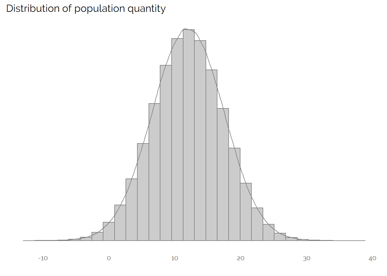
We can see that we have an approximately normally distributed variable, with a mean of 11.9973928. In most real examples, we wouldn’t be able to create this plot as we wouldn’t have access to data on the whole population.
One approach to understand this data set would be to take a random sample. If you can guarantee a true random sample (there is no response bias or other bias in your collection methodology) then this is a very effective approach. As explained in the paper, truly random sampling will dramatically increase your ability to accurately measure the quantity of interest.
If we take a random sample of 1,000 from our population of 1,000,000 and calculate the mean value of our quantity of interest as well as standard 95% confidence intervals we get the following:
##     CI_lwr     Mean   CI_upr
## 1 11.61331 11.95495 12.29658
The mean of this sample happens to be pretty close to the population figure, and the confidence interval covers a range which is just under 6% of the size of the mean value (i.e. we’re fairly confident in measuring the value to within +-3%).
As we have the population, we can take many different random samples and reproduce this process:
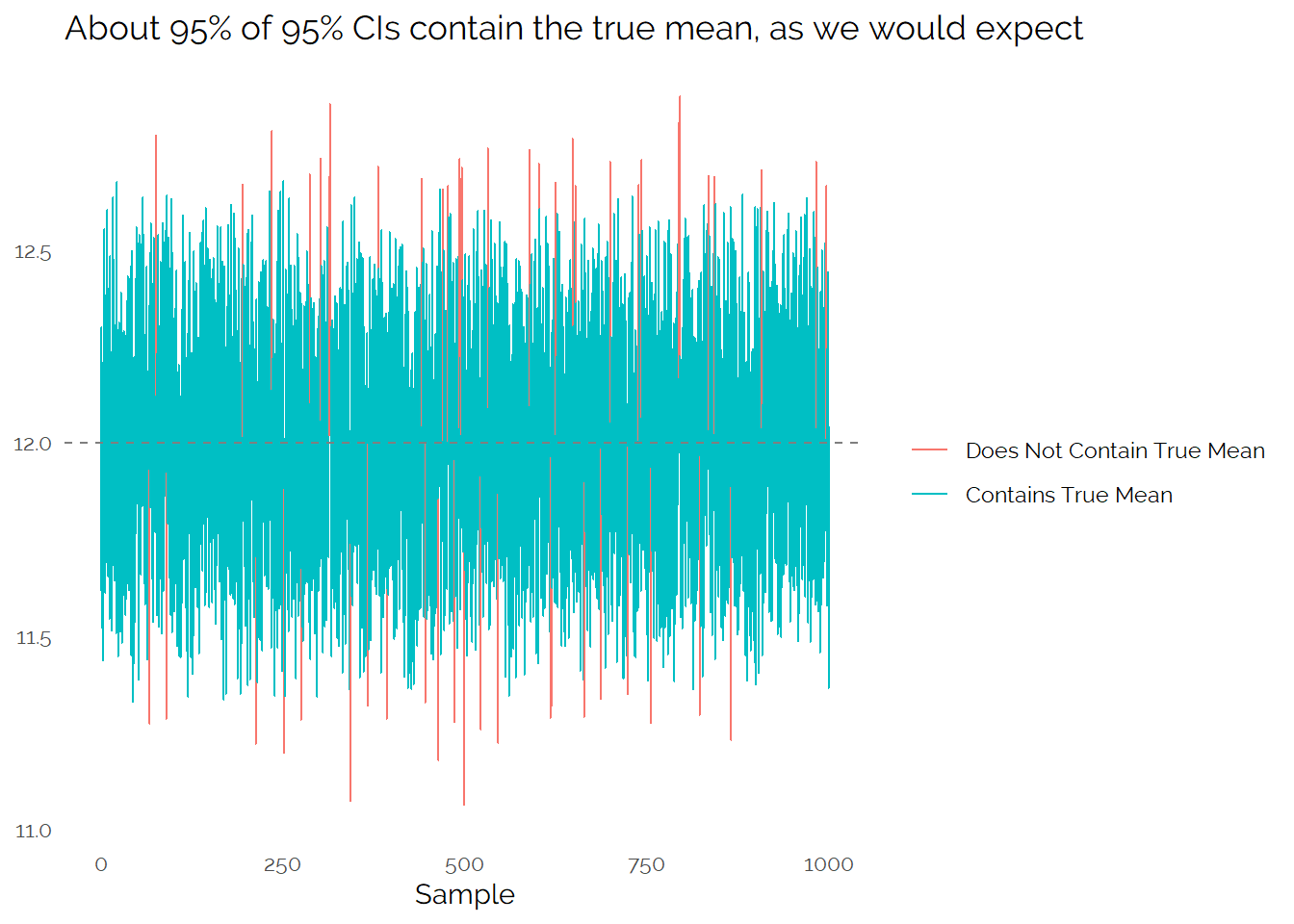
From this, we see that a random sample and the associated confidence interval will generally give us a good idea of what the true value is, but from a single sample there is a fair amount of uncertainty. If we get unlucky, our small sample might end up missing the true value we are trying to measure.
One way of trying to get around this challenge is to increase the sample size. Let’s imagine that we have a big sample of 800,000 which has some bias in how it is collected. What would we see from this?
##     CI_lwr     Mean   CI_upr
## 1 11.89834 11.91013 11.92193
Because of the large sample size, we have a very narrow confidence interval. However, in this case with a biased sample the confidence interval does not cover the true mean. By having a lot of data, but with an unknown and biased sampling scheme we may actually get misleading results.
If we take a large number of biased samples, we see that the confidence intervals never cover the true mean:
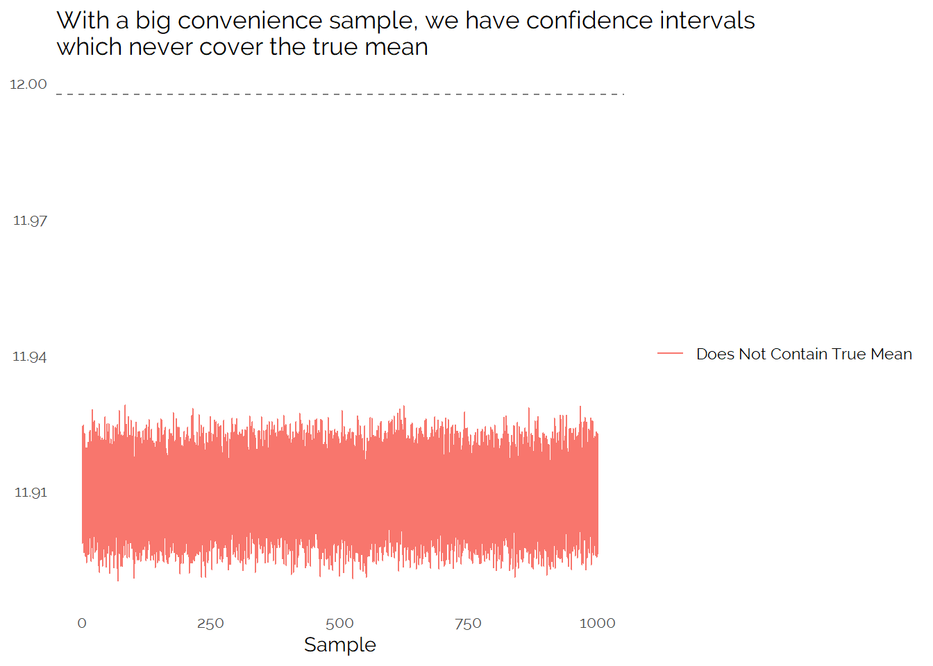
This shows that if we do not have a random sample, we cannot rely on standard confidence intervals to accurately cover the uncertainty in our measurement.
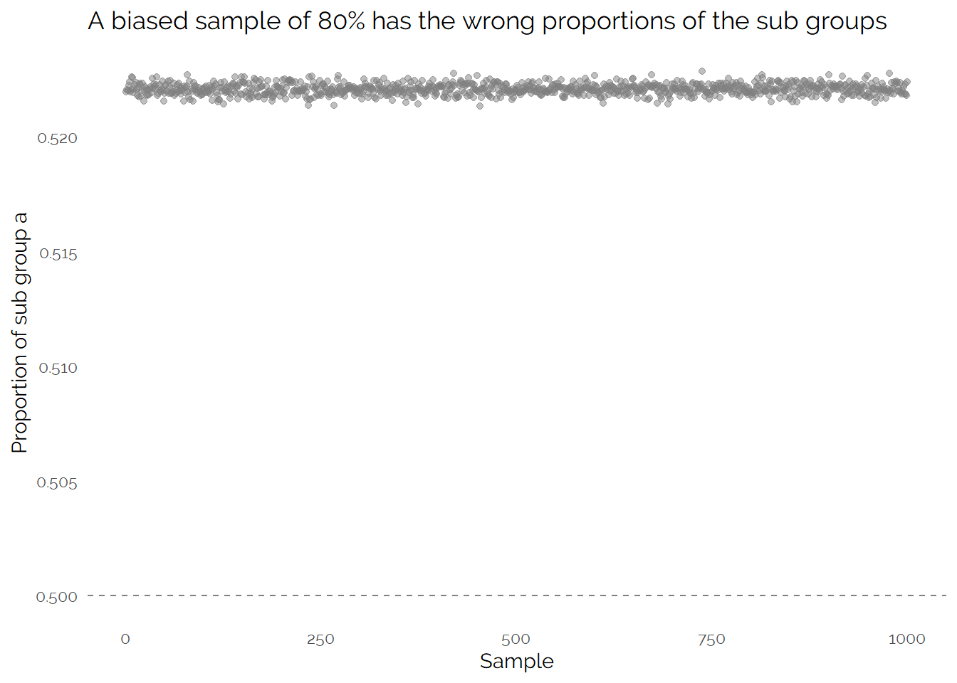
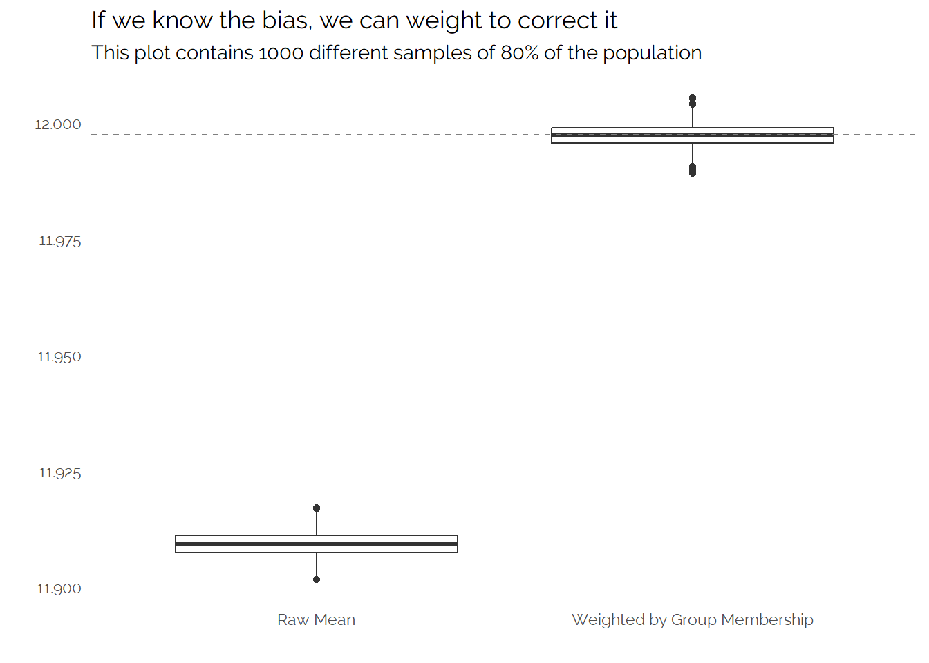
In this example, I have created the data so I know the generating process. The true population is made up of two evenly sized groups with different means and one group is about 1.4x more likely to be in my big sample than the other group. This results in a distorted population in the large sample:
Because we know the data generation process, we could create weights to get the correct proportions. Using multiple simulated samples to understand the uncertainty in our measurement (instead of relying on confidence intervals) we see that this is effective:
In the real world we often would not be able to directly measure the factors which cause a sampling or response bias. We often can measure a number of factors but these might not be a perfect way of unpicking the biases in our data. For example, if we have a sample of people we may know a number of “demographic” factors about these people such as their age or location, and while these factors may be correlated with what we want to measure (e.g. how profitable they are likely to be as a customer) and whether the individuals are in our convenience sample (how likely they are to consent to their data being collected) these factors won’t entirely explain the former or perfectly allow us to unpick the latter.
For this example, let’s imagine that we can’t ever measure the “group membership” which defines how the data is generated, so we cannot actually weight based on this factor. But we do have access to another binary variable, which we know is correlated with group membership.
As we have the population data, we can see the following:
## # A tibble: 2 x 2
##   group `Proportion with 1`
##   <chr>               <dbl>
## 1 a                   0.801
## 2 b                   0.200
So 80% of “group a” have a 1 for the trait we are able to measure, but only 20% of “group b” have this. In the overall population we see that 50.1% have a 1 for this trait, if we imagine that we know this population figure then we can instead weight to this.
If this sounds slightly abstract, then using the example from the paper to illustrate it might help. Consider the 2016 US Presidential Election. Donald Trump is a controversial and polarizing figure, and it appears that this might make people who support him less likely to respond to questionnaires asking their voting intentions. Whether you vote for Donald Trump or not is likely correlated how you have voted in previous elections (if you vote Republican once, you are more likely to vote that way next time). We know the result of the previous election, so can weight our respondents so they have the correct proportions of stated voting in past elections and use this as a way to hopefully get a more accurate proportion of Donald Trump supporters in our sample. However because this is not a perfect measure, and because people may not accurately remember or respond about their past voting behavior this is not going to perfectly fix the challenge.
The real world is more complicated than my simple example here, where I have only a single measure to weight with and a very simple approach to illustrating the challenge of trying to weight/debias the sample. But let’s see how effective it is with simulated data to weight our sample to get the correct proportions of the binary measure we can actually collect:
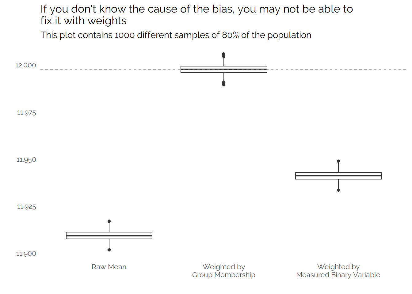
This helps make the results slightly better, but we are still under estimating the true mean and being over confident in our estimates due to the large sample.
By going through some relatively simple simulations, we have shown results which are inline with the paper whereby we see that a very large but biased sample gives results which are arguable less useful than a much smaller random sample, and that depending on what we can measure and weight to that weighting may not always be enough to fix the problem.
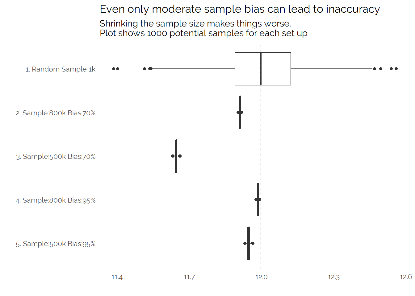
Let’s wrap up this post by looking at a few different simulated scenarios. The example above has a sample of 800,000 from the population of 1,000,000 where “group b” has a lower mean but each member is 0.7x less likely to be included in the sample. We can create a few different simulations with different assumptions and show the raw means:
My goal in this post was to try and simulate some data to explore the impact of biased sampling on the accuracy of measurement. Without getting into lots of detail, the findings seem to be consistent with the paper - having a lot of data isn’t enough to ensure that you can accurately measure something and it may actually mislead you if you treat biased data as if it is a random sample. Additionally, we can see some of the challenges in trying to make biased data look representative, if you can’t accurately measure the sources of bias then you cannot correct for them.
None of these topics are new, but it’s easy to forget about or underestimate the importance of random sampling when working with data, and it’s always good to be reminded to take more care about thinking what a data set really represents and what conclusions you can safely make from it.
The full code I used to generate the data looks as follows:
set.seed(123)

# Define the size of the population and two sub groups:
total_pop <- 1000000
prop_a <- 0.5
prop_b <- 1-prop_a

# Define means for the two different groups:
population_a <- rnorm(total_pop*prop_a,mean=10,sd=5)
population_b <- rnorm(total_pop*prop_b,mean=10*1.4,sd=5)

# define a binary variable which is correlated with group membership:
measurable_variable_a <- rbinom(total_pop*prop_a,1,0.8)
measurable_variable_b <- rbinom(total_pop*prop_a,1,0.2)

prop_measurable_variable_total <- sum(measurable_variable_a,measurable_variable_b) / total_pop

# Combine the data together:
data <- rbind(data.frame(mean=population_a,group="a", measurable_variable=measurable_variable_a, stringsAsFactors = F),
              data.frame(mean=population_b,group="b", measurable_variable=measurable_variable_b, stringsAsFactors = F))


# Define some weights to determine how relatively likely the two groups are to be included in the sample:

data %>%
  mutate(weight_1=if_else(group=="a",1,0.97),
         weight_2=if_else(group=="a",1,0.95),
         weight_3=if_else(group=="a",1,0.90),
         weight_4=if_else(group=="a",1,0.80),
         weight_5=if_else(group=="a",1,0.70),
         weight_n=if_else(group=="a",1,1)) -> data

# Make use of any parallel processing that is possible:
plan(multiprocess)

# Calculate Weighted/Raw Means based on a given sample size, and standard confidence intervals for raw values:
sample_and_calculate_statistics <- function(data, weight, size){

  data %>%
    mutate(random=runif(nrow(data)),
           order=random*{{weight}}) %>%
    arrange(-order) %>%
    filter(1:n()<=size) %>%
    ungroup() -> data

# First calculate weights using the known groups:
  data %>%
    group_by(group) %>%
    tally() %>%
    mutate(prop=n/sum(n)) -> group_weights

  group_weights %>%
    select(group,prop) %>%
    spread(key=group,value=prop) %>%
    rename(prop_a=a,
           prop_b=b) -> group_props

  group_weights %>%
    mutate(pop_prop=if_else(group=="a",prop_a,prop_b)) %>%
    mutate(group_weight=pop_prop/prop) %>%
    select(group,group_weight) -> group_weights

# Calculate weights using measurable_variable:
  data %>%
    group_by(measurable_variable) %>%
    tally() %>%
    mutate(prop=n/sum(n)) %>%
    mutate(pop_prop=if_else(measurable_variable==1,prop_measurable_variable_total,1-prop_measurable_variable_total)) %>%
    mutate(meas_weight=pop_prop/prop) %>%
    select(measurable_variable,meas_weight) -> meas_weights

  data %>%
    left_join(group_weights,by="group") %>%
    left_join(meas_weights,by="measurable_variable") %>%
    summarise(group_weighted_mean=sum(mean*group_weight)/sum(group_weight),
              meas_weighted_mean=sum(mean*meas_weight)/sum(meas_weight),
              raw_mean=mean(mean),
              CI_lwr=raw_mean-1.96*(sd(mean)/sqrt(n()-1)),
              CI_upr=raw_mean+1.96*(sd(mean)/sqrt(n()-1))) -> data

  cbind(data, group_props)
}


# Run all the simulations with different settings, using parallelism:

future_map_dfr(1:1000, ~sample_and_calculate_statistics(data,weight_n,size=800000), .progress=T) %>% mutate(experiment="wn_800")-> wn_800

future_map_dfr(1:1000, ~sample_and_calculate_statistics(data,weight_n,size=500000), .progress=T) %>% mutate(experiment="wn_500")->wn_500
future_map_dfr(1:1000, ~sample_and_calculate_statistics(data,weight_n,size=1000), .progress=T) %>% mutate(experiment="wn_1")-> wn_1

future_map_dfr(1:1000, ~sample_and_calculate_statistics(data,weight_2,size=800000), .progress=T) %>% mutate(experiment="w2_800") ->w2_800
future_map_dfr(1:1000, ~sample_and_calculate_statistics(data,weight_5,size=800000), .progress=T) %>% mutate(experiment="w5_800")-> w5_800
future_map_dfr(1:1000, ~sample_and_calculate_statistics(data,weight_2,size=500000), .progress=T) %>% mutate(experiment="w2_500")-> w2_500
future_map_dfr(1:1000, ~sample_and_calculate_statistics(data,weight_5,size=500000), .progress=T) %>% mutate(experiment="w5_500")-> w5_500

# Put all results into one data frame:
all_outputs <- rbind(wn_800,wn_500,wn_1,w2_800,w5_800,w2_500,w5_500)